Chapter 3 of Training Compute-Optimal Large Language Models
Estimating the Optimal Parameter/Token Allocation
Three independent approaches all converge on the same answer: N and D should scale equally.
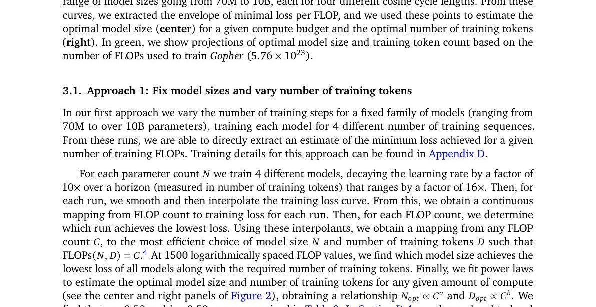 Fig. 2 — Training curve envelope (Approach 1): for each FLOP budget, the optimal model size (center) and training tokens (right) are extracted from the envelope of training loss curves across model sizes 70M–10B.
Approach 1 — Training Curve Envelope
For each model size (70M–10B parameters), train for 4 different token counts with a cosine schedule matched to each token count. For each FLOP budget, identify the (N, D) pair that achieves the lowest loss. Fit a power law to the envelope of optimal points.
Result: N_opt ∝ C^0.50, D_opt ∝ C^0.50
The key: every model uses a cosine schedule calibrated to its own training duration. This is what Kaplan et al. did not do.
Approach 2 — IsoFLOP Profiles
Fix 9 FLOP budgets (6×10^18 to 3×10^21). At each budget, vary model size and set training tokens so FLOPs = constant. Plot final loss vs. parameter count — a clear valley emerges. Fit a parabola to each valley to find the optimal N.
 Fig. 3 — IsoFLOP curves: each curve shows final loss vs. parameter count at a fixed compute budget. The valley gives N_opt for that budget.
Result: N_opt ∝ C^0.49, D_opt ∝ C^0.51
This approach directly answers: “for this FLOP budget, what is the optimal model size?” without interpolation.
Approach 3 — Parametric Loss Function
Model all final losses as:
L̂(N, D) = E + A/N^α + B/D^β
where:
- E = irreducible loss (entropy of natural language)
- A/N^α = capacity-limited excess loss (model too small)
- B/D^β = data-limited excess loss (insufficient training tokens)
Fit (A, B, E, α, β) by minimizing Huber loss (δ = 10^-3, robust to outliers) via L-BFGS over all 400+ runs. Grid initialization avoids local minima.
Efficient frontier (minimize L̂ subject to FLOPs ≈ 6ND):
Result: N_opt ∝ C^0.46, D_opt ∝ C^0.54
Approach 3 gives the most conservative (smallest) N_opt due to observed curvature in the frontier at high compute (see Appendix E).
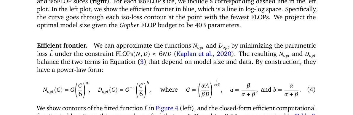 Fig. 4 — Parametric fit and efficient frontier: contour plot of L̂(N, D) (left) and isoFLOP slices (right). The efficient frontier (blue) is the Pareto-optimal boundary.
Summary — All Three Approaches vs. Kaplan et al.
| Approach | N_opt ∝ C^a | D_opt ∝ C^b |
|---|---|---|
| 1. Training curve envelope | 0.50 | 0.50 |
| 2. IsoFLOP profiles | 0.49 | 0.51 |
| 3. Parametric fit | 0.46 | 0.54 |
| Kaplan et al. (2020) | 0.73 | 0.27 |
Practical Look-Up Table (Approach 1)
| Model size | FLOPs required | Training tokens required |
|---|---|---|
| 1B | 1.21×10^20 | 20.2B |
| 10B | 1.23×10^22 | 205B |
| 67B | 5.76×10^23 (Gopher budget) | 1.5T |
| 175B | 3.85×10^24 | 3.7T |
| 280B | 9.90×10^24 | 5.9T |
| 520B | 3.43×10^25 | 11.0T |
A 175B-parameter model should be trained on 3.7 trillion tokens for compute-optimal training — 12× more than GPT-3 received. A 1T parameter model is not optimal unless the compute budget exceeds ~10^26 FLOPs (>250× Gopher).